PyPSA-Earth, end-to-end
A forensic walkthrough of Falgun Associates' Bangladesh model — every data source, every script, every output, and how it stitches together. Built for Karim, refreshed 2026-05-04 against the live team repo.
1 · What PyPSA-Earth actually is
PyPSA-Earth is a global, open-source energy-system optimisation framework built on top of PyPSA (Python for Power System Analysis). It reduces the question “how should this country decarbonise?” to a single Linear Program:
It's capacity expansion + dispatch at the same time. The optimiser doesn't just pick what to build — it co-optimises where on the grid, how often each plant runs, and how electricity / heat / gas / hydrogen flow between zones.
The four building blocks
① Snakemake DAG
The whole workflow is a Snakemake pipeline (a Python DSL like a Makefile). Each rule = one Python script with declared inputs/outputs. Snakemake figures out execution order from the DAG.
② PyPSA network object
An in-memory graph of buses, lines, links, generators, loads, storage_units, stores. Saved as NetCDF (.nc). Every script either builds or augments this object.
③ Atlite weather cutout
An ERA5 NetCDF block of every weather variable (wind, GHI, temperature, runoff) for the country bounding box × the simulation year. Renewables potentials are derived from this.
④ Linopy + a solver
Linopy formulates the LP. The solver (Gurobi here; HiGHS as fallback) finds the optimum. Solution is written back into p_nom_opt, dispatch timeseries, etc.
What “sector-coupled” means here
Vanilla PyPSA-Earth was electricity-only. The sector-coupled variant adds, as additional carriers and links on the same graph:
- Heat — residential / services / industrial low-temp via heat pumps, resistive heaters, gas boilers, CHP, district heating
- Land transport — ICE oil load + EV charging links + V2G + fuel-cell vehicles
- Industry — process heat (low/high T), feedstock (naphtha, methanol), industrial CCS
- Hydrogen — electrolysis, fuel cell, pipelines (off in BD), salt caverns (none in BD)
- CO₂ accounting — atmosphere ↔ stored CO₂ buses, DAC, biomass-with-CCS
- Agriculture, biomass — crop residues, biogas potential, machinery oil
So a single LP simultaneously decides whether to electrify a steel plant, whether to build a heat pump or keep a gas boiler, and whether to import LNG or build an electrolyser.
2 · The pipeline, rule by rule
The Snakemake DAG runs in three stages. Each box below is a script in pypsa-earth/scripts/. Arrows show what feeds what.
networks/base.nc — empty PyPSA graph with only buses + lineselec.nc — base + powerplants + RE profiles + loads + costselec_s.nc — collapse parallel lines, dissolve transformers, keep just ACelec_s_{N}.nc — k-means or GADM-based clustering down to N buses (8 here, 10 in pre-built BD)elec_s_{N}_ec.nc — battery + H₂ stores/links per buselec_s_{N}_ec_l{ll}_{opts}.nc — applies CO₂ cap, line-volume cap, time aggregation (e.g. Co2L-3h)results/networks/... — electricity-only solved LP. First decision point: does the elec grid even balance under the cap?urban_percent.csv)prenetworks/... — adds heat / transport / industry / H₂ buses+links to the clustered electricity networkh2export: [0])postnetworks/...nc — solves the LP for that horizon's prenetwork; output becomes the brownfield input for the next horizonThe wildcard system (how Snakemake parameterises a run)
| Wildcard | Meaning | This run |
|---|---|---|
{simpl} | Simplification level (HAC merging) | "" (none) |
{clusters} | Number of buses after clustering | 8 (GADM-1) |
{ll} | Line-volume cap: copt=optimum, v1.0=fixed at base | copt |
{opts} | Constraint string (e.g. Co2L-24H) | Co2L-24H |
{sopts} | Sector-coupled time resolution | 24h |
{planning_horizons} | Which year is being solved | 2030, 2040, 2050 |
{discountrate} | Real discount rate | 0.071 |
{demand} | SSP demand scenario | AB (SSP2 moderate) |
{h2export} | H₂ export demand (TWh) | 0 |
So the canonical filename of a final solved BD network is:
results/Case_NetZero2050_NDC/postnetworks/elec_s_8_ec_lcopt_Co2L-24H_24h_2050_0.071_AB_0export.nc
3 · Data sources — the complete inventory
Every external dataset PyPSA-Earth touches, what it's used for, and where it lives in our copy.
Geospatial & weather
| Source | What & why | File(s) |
|---|---|---|
| GADM 4.1 | Country + division polygons. The clustering uses GADM-1 (8 BD divisions) instead of k-means. | data/3_bangladesh_data/gadm/gadm41_BGD/gadm41_BGD.gpkg |
| GEBCO 2025 | Global bathymetry — used to mask offshore wind (max_depth: 50 m). | data/2_global_geodata/gebco/GEBCO_2025_sub_ice.nc |
| HydroBASINS lvl 6 | Watershed polygons — feed Atlite's hydro inflow model (flowspeed 1 m/s). | data/2_global_geodata/hydrobasins/hybas_*_lev06_v1c.shp |
| Copernicus PROBAV LC100 | Global land-cover raster (100 m). Excludes urban (50), water (80) etc. for RE potentials. | data/2_global_geodata/copernicus/PROBAV_LC100_global_v3.0.1_2019-nrt_*.tif |
| Marine Regions EEZ v11 | Exclusive Economic Zones — bounds offshore wind buildable area. | data/2_global_geodata/eez/eez_v11.gpkg |
| Natura 2000 | Protected-area mask. Included tif (natura: true) excludes RE in those cells. | data/2_global_geodata/natura/natura.tiff |
| WorldPop 2020 1 km (UN-adj, constrained) | Population raster — underpins the urban/rural split, demand allocation, GDP layouts. | data/3_bangladesh_data/WorldPop/bgd_ppp_2020_UNadj_constrained.tif |
| OSM (BD planet extract) | HV grid skeleton (≥51 kV substations, lines, cables) and OSM-listed power plants. | data/3_bangladesh_data/osm_pbf/bangladesh-latest.osm.pbf |
| OSM Power JSON | Pre-extracted BD power infrastructure (substations, lines, generators). | data/3_bangladesh_data/osm_power/BD_power.json |
| Microsoft Global ML Buildings | Building footprints — used by solar_rooftop (currently disabled — IncompleteRead errors). | data/3_bangladesh_data/global_buildings/ |
| ERA5 (Copernicus CDS) | Hourly weather cutout (wind, GHI, T, runoff) — the entire RE potentials story. | missing — must rebuild via CDS API or get from Paul |
| SSP scenarios | Per-cell load projections under SSP1–5 (we use SSP2-2.6). | data/2_global_geodata/ssp2-2.6/{2030,2040,2050,2100}/ |
Energy / techno-economic data
| Source | What & why | File(s) |
|---|---|---|
| UN Statistics Division Energy DB | National-level energy balances by carrier and use; basis for sectoral demand split. | data/4_reference_csvs/demand/unsd/data/UNdata_Export_*.txt (double-extracted at two timestamps in the zip — use the newer one) |
| IEA Bangladesh portal | National generation by source, TES, low-carbon share. | data/IEA Energy Supply by Source/*.csv |
| IRENA capacity stats | Reference renewable installed capacity by country (used by estimate_renewable_capacities, year 2023). | fetched at runtime via powerplantmatching |
| technology-data v0.13.2 (DEA / Fraunhofer / NREL) | CAPEX, FOM, VOM, lifetime, efficiency, fuel cost for every tech, per year. | resources/costs_2030.csv, costs_2040.csv, ... generated from raw.githubusercontent.com/PyPSA/technology-data/v0.13.2 — but disabled here (retrieve_cost_data: false) in favour of BD-specific costs. |
| BPDB / IEPMP 2023 | Bangladesh-specific cost data feeding the LP — overrides the DEA defaults. Mentioned in config comments. | data/costs_*_bd.csv (referenced; ship as resources/costs_{year}.csv) |
| IEA Hydro annual generation | Used to rescale Atlite's hydro inflow to match observed annual energy. | data/4_reference_csvs/eia_hydro_annual_generation.csv |
| Custom industrial database | Coordinates & capacity of cement, steel, paper, aluminium plants — input to industrial distribution key. | data/4_reference_csvs/industrial_database.csv (partial BD coverage) |
| SFI cement / pulp&paper databases | Source data for the industrial database. | data/4_reference_csvs/industry/SFI-Global-Cement-Database-July-2021.xlsx + SFI_ALD_Pulp_Paper_Sample_LatAm_Jan_2023.xlsx |
| Aluminium production | Annual primary Al demand (year 2019 here). | data/4_reference_csvs/AL_production.csv |
| BDEW heat-load profile (Germany) | Standard hourly heat-demand shape, scaled to local annual totals. ⚠ German shape — see caveats. | data/4_reference_csvs/heat_load_profile_BDEW.csv |
| Hydro capacities | EIA dataset — country totals for hydro / PHS power and energy. | data/4_reference_csvs/hydro_capacities.csv |
| European car ownership (e-mobility) | Per-capita car-stock used to scale transport demand. | data/4_reference_csvs/emobility/European_countries_car_ownership.csv |
| Custom powerplants (Nahid & Roy 2025) | BPDB-validated list of operating BD powerplants with retrofit/retire dates — replaces the auto-fetched OSM2PM list (custom_powerplants: replace). | data/custom_powerplants.csv |
| SSP CAGR tables | Per-sector growth + efficiency-gain compound-annual rates used to project demand to 2030/40/50. | data/4_reference_csvs/demand/{efficiency_gains_cagr.csv, growth_factors_cagr.csv, industry_growth_cagr.csv, fuel_shares.csv} ⚠ no BD row — falls back to “default” which is Morocco's curve. |
Configuration files
| File | Purpose |
|---|---|
configs/config.yaml | The run config — overrides config.default.yaml. This is the only file that matters day-to-day. |
configs/config.default.yaml | Upstream defaults (every key documented here). |
configs/bundle_config.yaml | Lists data bundles + Zenodo/Drive URLs for retrieve_databundle. Disabled here. |
configs/regions_definition_config.yaml | OSM column types + ISO-2/world region map. |
configs/powerplantmatching_config.yaml | Overrides for the powerplantmatching package (custom replace policy). |
4 · Bangladesh customisations (team's diff)
Live source: bet/pypsa-earth/config.yaml on team repo's main branch (HEAD d9f44f3). Two scenario overlays apply on top:
| Scenario | configfile | Storyline |
|---|---|---|
Case_BAU_NDC | configs/scenarios/config.bau.yaml | No climate policy. CO₂ unconstrained; emissions emerge from cost-min. Used to compare model BAU vs NDC 3.0 BAU (272 Mt 2035). |
Case_NetZero2050_NDC | configs/scenarios/config.nz.yaml | NDC-aligned through 2035, net-zero by 2050. |
snakemake --configfile config.yaml --configfile configs/scenarios/config.nz.yaml ...
① Geographic + temporal scope
["BD"]
snapshots2013-01-01 → 2014-01-01 (left-inclusive)
weather year2013 (ERA5)
foresightmyopic (sequential per horizon)
planning_horizons[2030, 2035, 2050] — NDC-anchored
opts / soptsCo2L-24H + 24h → 365 daily snapshots/horizon
clusters8 = GADM-1 divisions (alternative_clustering: true)
② CO₂ trajectory (custom block, scenario-dependent)
BAU (config.bau.yaml): co2_budget.enable: false; electricity.co2limit: 1e+12 (effectively unbounded).
NetZero 2050 NDC (config.nz.yaml):
co2_budget:
  enable: true
  year:
    2030: 2.55   # 248 MtCO2 (NDC 3.0 emissions peak)
    2035: 2.32   # 225 MtCO2 (NDC 3.0 conditional commitment)
    2050: 0.05   #   5 MtCO2 (1.5 °C-aligned net-zero endpoint)
Fractions multiply electricity.co2limit = 9.7 × 10⁷ tCO₂/yr (IEA 2020 BD baseline). Fractions > 1 reflect absolute budgets above 2020 levels — required because BD emissions are still rising.
CLAUDE.md still references the older AllSector_Brownfield design (4 horizons 2030/2040/2050/2065, fractions 1.0/0.65/0.20/0.05). The latest already-solved results in that doc come from that design. The two-scenario NDC pivot above is from commit e30053f "Add two-scenario NDC-anchored model design" — not yet re-solved as of repo HEAD.
③ Sector flags — Phase-1 set
| On | Off | Why off |
|---|---|---|
heat, biomass, industry, land_transport, residential, services, agriculture |
shipping, aviation, rail_transport |
<0.3 % of national emissions; cause NaN issues for non-port nodes |
| On | Off | Why off |
|---|---|---|
tes, chp, solar_thermal, boilers, biomass_transport, dac, cc | v2g, bev_dsm, solar_rooftop, electricity_distribution_grid, home_battery, methanation, fischer_tropsch, SMR, SMR CC, helmeth, oil_boilers, micro_chp | Phase 1 — minimise spatial-link explosion; solar_rooftop has flaky download |
gas.spatial_gas: true, oil.spatial_oil: true, coal.spatial_coal: true | gas.network, hydrogen.network, co2_network, lignite.spatial_lignite | BD has no GGIT pipeline data; spatial H₂/CO₂ networks add huge link counts |
④ Custom industry-decarbonisation block (not vanilla — likely Paul's branch)
sector.industry_decarbonisation:
  coal_to_gas: true   # gas substitutes industrial coal
  coal_to_elec: true  # electric process heat replaces coal
  oil_to_gas: true
  oil_to_elec: true
When enabled, industrial coal/oil emissions become optimisable links rather than fixed loads — the LP gets to fuel-switch on the cost curve. This block is not in the public pdockery/pypsa-earth tree — it lives on an unpushed branch.
⑤ Existing-fleet treatment
replace (use the BPDB-validated list)
powerplants_filter(DateOut ≥ 2022 or DateOut != DateOut) — drops plants already retired
allow_early_retirementtrue — optimiser can retire a unit before end-of-life if the LP justifies it
keep_existing_capacitiestrue — 2030 starts from the actual ~38 GW fleet, not a blank slate
estimate_renewable_capacities.statsirena, year 2023, p_nom_min: 1 (lock current installed RE in)
⑥ Numerical tuning for BD's bad scaling
BD cost data spans a 6 × 10⁹ range (very small marginal costs vs. very large investments). Default Gurobi diverges. The config switches to a custom gurobi-numeric-focus profile:
NumericFocus: 3        # stability over speed
ScaleFlag:    2        # aggressive matrix scaling
BarHomogeneous: 1      # fall back to homogeneous barrier
DualReductions: 0      # don't claim "infeasible_or_unbounded" on H2 export bus
BarConvTol: 1e-4       # relaxed tolerances
FeasibilityTol: 1e-4
OptimalityTol: 1e-4
5 · Inside the BAU + NetZero2050_NDC runs
What the optimiser is actually computing, in plain language.
Decision variables
| Variable family | Per | Bounds |
|---|---|---|
Generator.p_nom (capacity) | tech × bus | [p_nom_min, ∞] (or fixed if extendable: false) |
Generator.p (dispatch) | tech × bus × snapshot | [0, p_max_pu × p_nom] |
StorageUnit.p_dispatch / p_store / state_of_charge | bus × snapshot | storage capacity, max_hours |
Store.e (energy state) | bus × snapshot | 0 ≤ e ≤ e_nom |
Line.s_nom | line | fixed at base × line-volume cap (here: copt = optimum subject to global cap) |
Link.p_nom + Link.p | link × snapshot | e.g. heat pumps, electrolysers, fuel cells |
Constraints (the LP wall)
- Nodal energy balance at every bus, every snapshot: generation + storage discharge − storage charge − load + net imports = 0
- Kirchhoff for AC lines (PTDF formulation)
- Capacity factors:
p ≤ p_max_pu(t) × p_nom(RE) orp ≤ availability × p_nom(thermal) - Storage state evolution:
SoC(t) = η · SoC(t-1) + p_charge − p_discharge - Global CO₂ cap: Σ (carrier emission factor × dispatch) ≤
co2limit × fraction(year) - Line-volume cap: Σ
length × s_nom≤line_volume_cap - Sector links: heat-pump COP timeseries, electrolyser efficiency, EV-charger availability windows, biomass-transport costs
Objective
min  Σ_techs ( annuity(CAPEX) × p_nom + FOM × p_nom )
   +  Σ_techs,t ( marginal_cost(t) × p(t) )
   +  Σ_lines  ( line CAPEX × s_nom )
   +  Σ_co2    ( emission_price × emissions )
“Annuity” converts CAPEX into a per-year cost using the discount rate (0.071) and tech lifetime. So we're minimising annual system cost in 2030 / 2040 / 2050, separately, with each horizon's solution feeding the next as fixed brownfield.
Myopic foresight, in pictures (NetZero2050_NDC)
2030 horizon:
  - existing fleet (~38 GW, DateOut ≥ 2022)        → fixed
  - extendable: solar, onwind, OCGT, CCGT, batteries, H2…
  - CO2 cap = 2.55 × 9.7e7 = 248 Mt   (NDC 3.0 peak; budget grows because emissions still rising)
  - SOLVE → p_nom_opt[2030]

2035 horizon:
  - p_nom_opt[2030] is now BROWNFIELD (fixed)      ← add_brownfield
  - retire what aged out
  - new build optimised on top
  - CO2 cap = 2.32 × 9.7e7 = 225 Mt   (NDC 3.0 conditional commitment)
  - SOLVE → p_nom_opt[2035]

2050 horizon:
  - p_nom_opt[2030] + p_nom_opt[2035] BROWNFIELD
  - CO2 cap = 0.05 × 9.7e7 = 5 Mt     (1.5 °C-aligned net-zero endpoint)
  - SOLVE → p_nom_opt[2050]
Myopic ≠ optimal-overall. The 2030 LP doesn't know 2050's cap is 95 % cut — it only sees its own 10 % cap. So you can get short-sighted gas build-out in 2030 that becomes stranded in 2050. That's by design; it mimics how real planners decide. Perfect-foresight (Case3, future) would avoid it.
6 · Outputs — what comes out, how to read it
Latest already-solved results (from team's CLAUDE.md, AllSector_Brownfield run)
| Year | Cost (€B) | CO₂ (Mt) | Strategy | CO₂ stored (Mt) |
|---|---|---|---|---|
| 2030 | 3.74 | 97.0 | Status quo | 0 |
| 2040 | 8.06 | 63.0 | Coal/oil CC | 58.9 |
| 2050 | 11.88 | 19.4 | Full CC, gas out | 136.3 |
| 2065 | 26.81 | 4.85 | CC + electrification | 200.0 (limit) |
These were produced under the older 4-horizon AllSector_Brownfield design. The two-scenario NDC pivot (BAU + NetZero2050_NDC, 3 horizons) is freshly committed but not yet re-solved.
The headline files per horizon (current NDC design)
| File | What's in it |
|---|---|
postnetworks/elec_s_8_ec_lcopt_Co2L-24H_24h_2030_0.071_AB_0export.nc | Solved network for 2030 — capacities, dispatch, emissions, prices |
postnetworks/...2035...nc | 2035 (with 2030 as brownfield) |
postnetworks/...2050...nc | 2050 (with 2030+2035 as brownfield) |
summaries/elec_s_8...csv | Costs / capacities / energy / emissions tabulated across horizons |
maps/...pdf | Geographic plots — capacity by node, line flows, costs |
graphs/{costs,energy,balances-energy}.pdf | Stacked-bar timelines |
How to read a solved network in Python
import pypsa
n = pypsa.Network("results/Case_NetZero2050_NDC/postnetworks/...2050_0.071_AB_0export.nc")

# Capacities
n.generators.groupby("carrier").p_nom_opt.sum() / 1e3   # GW per tech, year 2050
n.links.groupby("carrier").p_nom_opt.sum() / 1e3        # heat pumps, electrolysers…
n.stores.groupby("carrier").e_nom_opt.sum() / 1e6       # TWh of H2 / battery storage

# Dispatch
n.generators_t.p.sum() * n.snapshot_weightings.objective.iloc[0] / 1e6  # TWh/year
n.statistics.energy_balance().round()                   # full sectoral balance

# Costs
n.statistics.capex().round()                            # €/yr CAPEX by tech
n.statistics.opex().round()                             # €/yr OPEX by tech
n.statistics.installed_capex().round()                  # one-off €

# Emissions
n.global_constraints                                    # CO2 cap + shadow price
n.generators_t.p.mul(n.generators.carrier.map(n.carriers.co2_emissions))
The 8 buses
With alternative_clustering: true + gadm_layer_id: 1, the 8 buses are the GADM-1 divisions:
| NAME_1 | Population (M) | Modelled demand share |
|---|---|---|
| Dhaka | ~45 | 26 % |
| Chittagong | ~32 | 19 % |
| Rajshahi | ~20 | 14 % |
| Rangpur | ~17 | 10 % |
| Khulna | ~16 | 17 % |
| Mymensingh | ~12 | (0 % — clustering artefact, see caveats) |
| Sylhet | ~12 | 5 % |
| Barisal | ~8 | 10 % |
7 · Karim outputs — first results off the network
Run on pypsa-bd/networks/elec_s_10*.nc (Paul's pre-built BD network, 10 buses, 2013 hourly).
Source scripts in karim_outputs/scripts/.
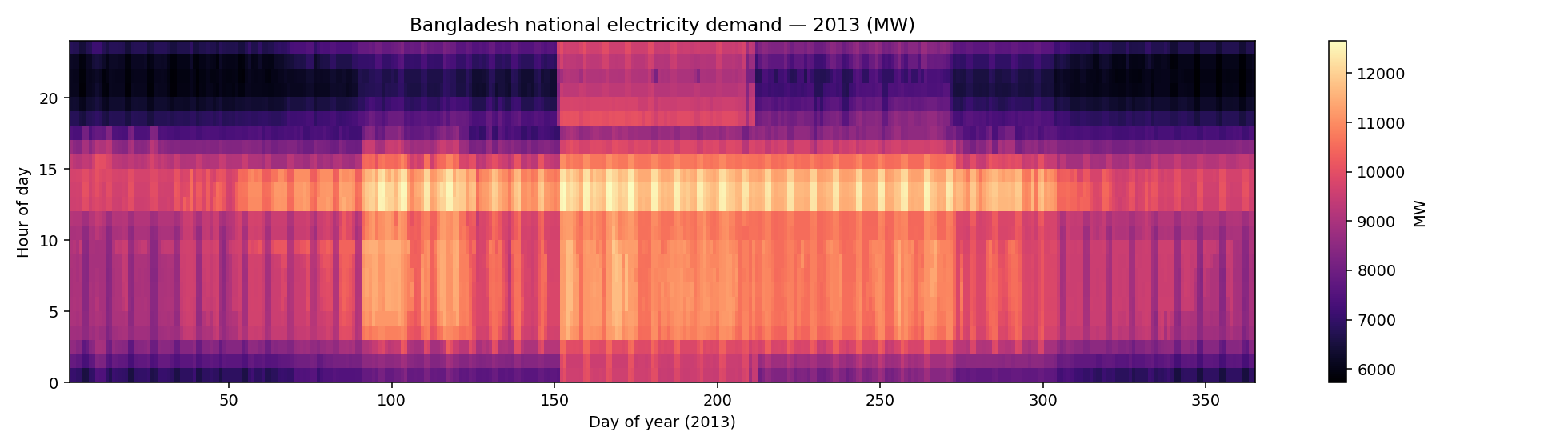
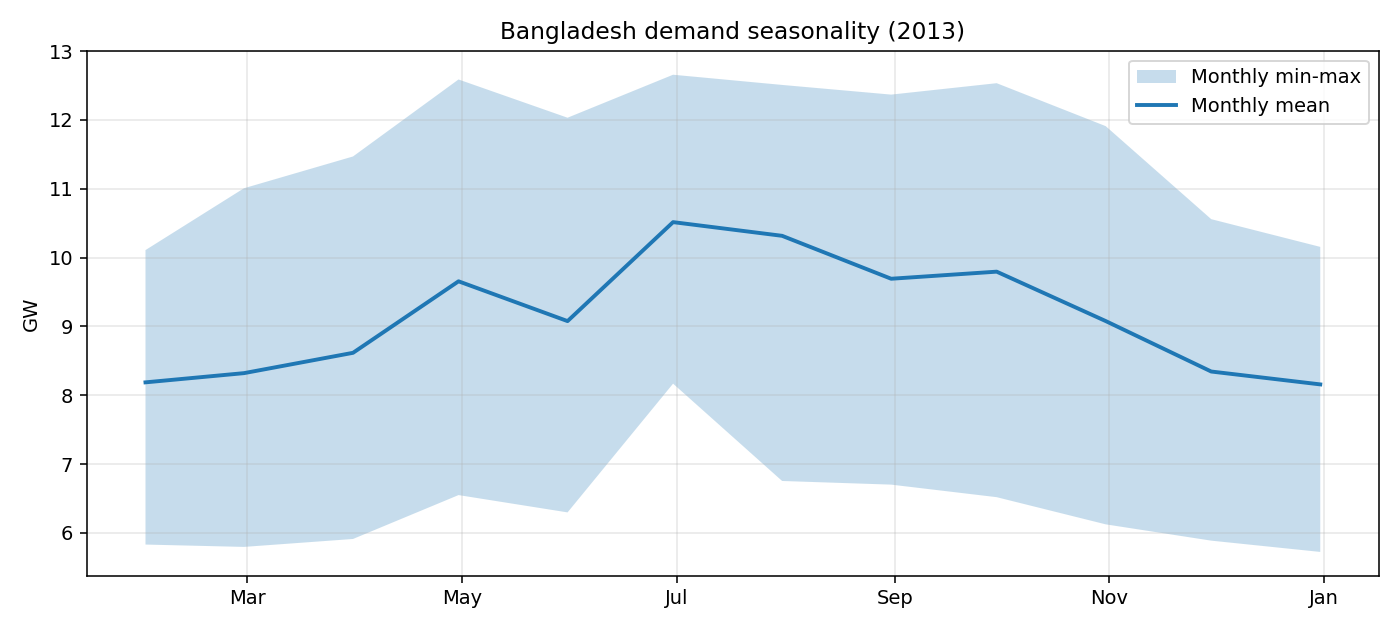
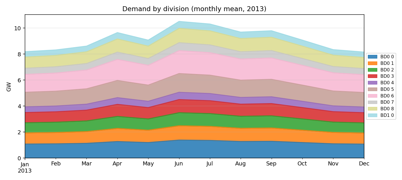
Demand fundamentals

Transmission stress — moved to simulation/HV_power_flow.ipynb
Originally analysed here off the pandapower snapshot. Now consolidated into bet/simulation/HV_power_flow.ipynb which reads solved post-networks for each horizon. Headline finding from the AllSector_Brownfield results in data/6_results/:
| Scenario · year | Max loading | Mean loading | Lines > 70 % |
|---|---|---|---|
| AllSector 2030 | 43.6 % | 17.9 % | 0 |
| AllSector 2040 | 80.0 % | 37.4 % | 4 |
| AllSector 2050 | 80.0 % | 40.8 % | 5 |
| AllSector 2065 | 80.0 % | 38.2 % | 6 |
The 80 % ceiling is the s_max_pu config cap — multiple lines hitting it from 2040 onward means binding transmission constraints emerging as the system decarbonises. Open the notebook to see the full-year loading histograms, per-division stress, and the geographic max-loading map.
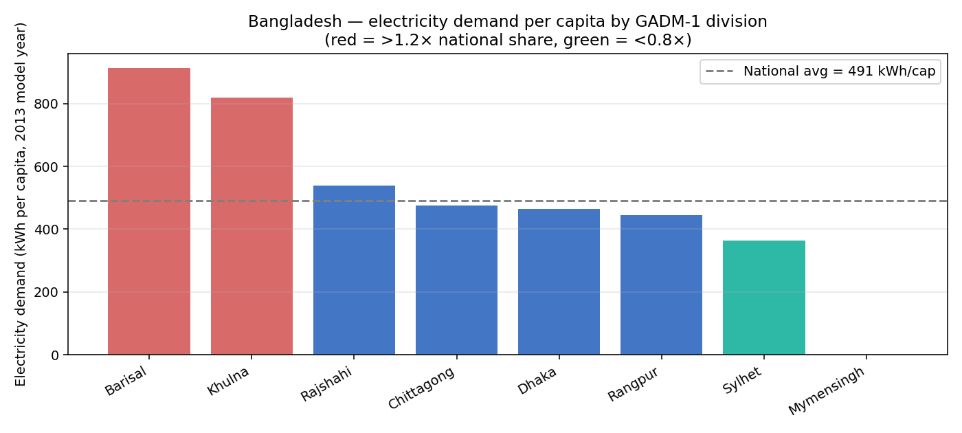
Equity — demand per capita by division
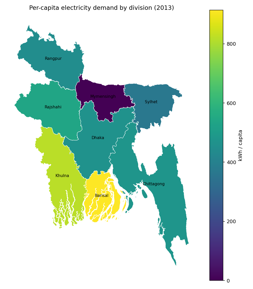
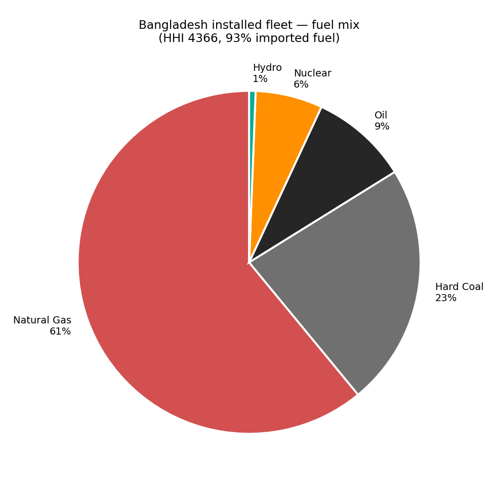
Energy security — fleet composition & concentration
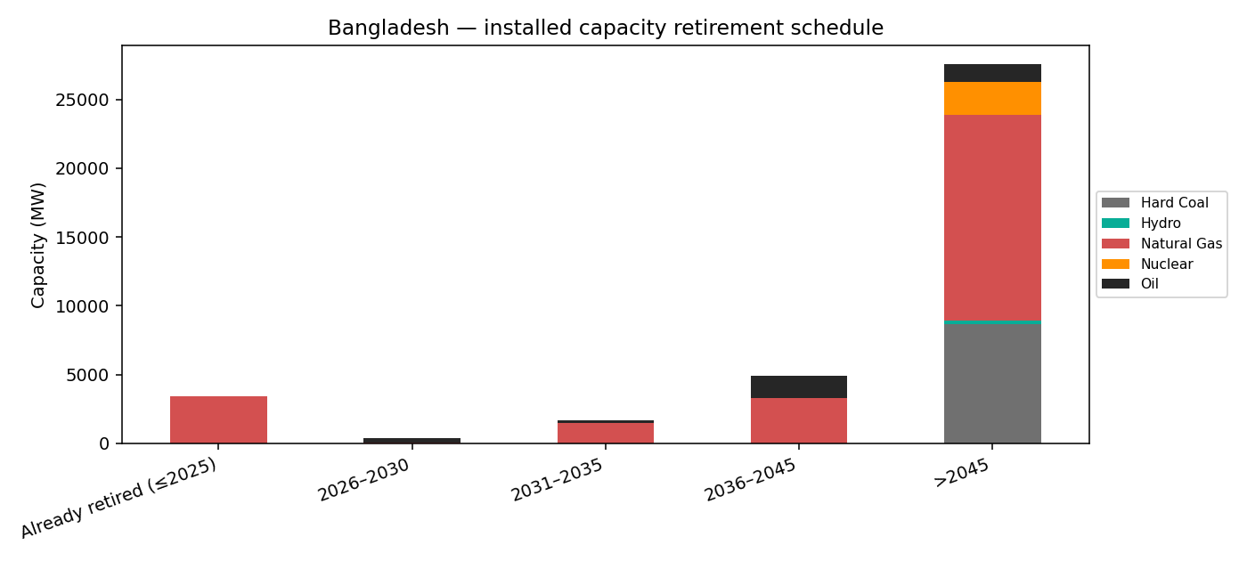
DateOut (≤2025). Replacement window opens immediately.8 · Data caveats & open issues
Four reference CSVs have no Bangladesh row —
efficiency_gains_cagr.csv, growth_factors_cagr.csv, industry_growth_cagr.csv, fuel_shares.csv. The loader silently falls back to the row labelled default, which is parameterised on Morocco. This means BD's residential heat demand grows on a Moroccan curve unless we add a BD-row override.
heat_load_profile_BDEW.csv is a German residential heat-demand shape (BDEW H0). BD has effectively no space-heat — “residential heat” here is mostly cooking/water. The BDEW shape will misrepresent both magnitude and timing. Worth a sensitivity.
data/4_reference_csvs/costs.csv is 2010–2013 vintage. The config disables retrieve_cost_data and points at BD-specific costs — but those need verification (IEPMP 2023 / BPDB sources). Renewable CAPEX in particular has dropped >60 % since 2013.
The bundled
industrial_database.csv has partial BD coverage. The pulp/paper and cement files in data/4_reference_csvs/industry/ are LatAm samples, not BD. Industrial heat demand is therefore dispatched against an under-specified node-level industrial layout.
The OneDrive export skipped
Data/1_cutouts (see ___All_Errors.txt). Without it, build_renewable_profiles, build_temperature_profiles, build_solar_thermal_profiles, and build_heat_demand all fail. Two fixes: (a) get a Copernicus CDS API key and run build_cutout (~30 min for BD bbox × 2013); (b) request the file from Paul.
Earlier versions of this page assumed the model lived on Paul's
pdockery/pypsa-earth fork. The authoritative source is now wilhem-hector/bangladesh_energy_transition (main branch). It carries the full custom code — industry_decarbonisation, override_co2opt, the scenario configfiles, the brownfield/baseyear fixes, the LaTeX writeup, and the visualisation notebook.
The team's
CLAUDE.md still describes the older AllSector_Brownfield design (4 horizons 2030/2040/2050/2065). The live config.yaml + configs/scenarios/config.{bau,nz}.yaml have moved to a 3-horizon NDC-anchored design (2030/2035/2050) with two scenarios. Anyone reading CLAUDE.md before running will reach for the wrong scenario name. Worth flagging to Hector / Paul.
The pre-built
elec_s_10 network has 10 PyPSA buses, but they don't centroidally fall inside all 8 GADM-1 polygons. Mymensingh has no PyPSA bus → zero demand allocated. If that bus mapping survives into the GADM-1 (8-cluster) run, equity analysis will mis-attribute. Verify after the GADM-1 run is solved.
download_global_buildings keeps failing with IncompleteRead timeouts → solar_rooftop: false. So distributed PV potential is excluded from the LP. Given Bangladesh's million-solar-home-systems history, this is a meaningful omission for both equity and security narratives.
Generated for Falgun Associates, refreshed 2026-05-04.
Local workspace: /Users/karimarnous/FalgunXBangladesh.
Team repo (canonical): wilhem-hector/bangladesh_energy_transition.
Karim outputs: bet/karim_outputs/.